Soft-Margin SVM
In order to avoid the effect of noise in dataset, we allow the model to make a small number of mistakes, similar to PLA, we have a new optimization goal shaped like
\[\begin{split} \min_{b,\boldsymbol w} \ \ &\frac{1}{2}\boldsymbol w^\text T\boldsymbol w+C \cdot \sum_{n=1}^N[\![y_n \ne \text{sign}(\boldsymbol w^\text T\boldsymbol x+b)]\!] \\[1em] \text{s.t.} \ \ &y_n(\boldsymbol w^\text T\boldsymbol x_n+b)\ge 1-\infty \ \cdot [\![y_n \ne \text{sign}(\boldsymbol w^\text T\boldsymbol x+b)]\!], \ n=1,2,...,N \end{split} \tag{9.31}\]the constraint means we only care about points separated correctly, for these error point we take them into the penalty in our goal and use constant $C$ to set our tolerance for errors. However, there are two cons of our model. Firstly it is non-linear, and secondly the penalty of this model cannot distinguish points with small error or large error. In order to solve the two problems, we modify our goal as follows:
\[\begin{split} \min_{b,\boldsymbol w,\boldsymbol\xi} \ \ &\frac{1}{2}\boldsymbol w^\text T\boldsymbol w+C \cdot \sum_{n=1}^N\xi_n \\[1em] \text{s.t.} \ \ &y_n(\boldsymbol w^\text T\boldsymbol x_n+b)\ge 1-\xi_n \\[1em] &\xi_n \ge 0, \ n=1,2,...,N \end{split} \tag{9.32}\]where $\xi_n$ describes the ‘margin violation’ , in other words the degree of error in sample point.
Next we construct Lagrange dual problem similar as before. With an increased constraints, we set two Lagrange multipliers $\alpha_n$ and $\beta_n$. Then we have Lagrange function
\[\mathcal L(b,\boldsymbol w,\boldsymbol\xi,\boldsymbol\alpha,\boldsymbol\beta) = \frac{1}{2}\boldsymbol w^\text T\boldsymbol w+C \cdot \sum_{n=1}^N\xi_n + \sum_{n=1}^N\alpha_n\left(1-\xi_n-y_n(\boldsymbol w^\text T\boldsymbol x_n+b)\right) + \sum_{n=1}^N\beta_n(-\xi_n) \tag{9.33}\]and the dual problem is
\[\max_{\alpha_n \ge 0, \beta_n \ge 0} \ \min_{b,\boldsymbol w,\boldsymbol\xi} \ \ \mathcal L(b,\boldsymbol w,\boldsymbol\xi,\boldsymbol\alpha,\boldsymbol\beta) \tag{9.34}\]Firstly, we set $\nabla_{\xi_n}\mathcal L = 0$, we have
\[C-\alpha_n-\beta_n=0 \tag{9.35}\]which means we can eliminate $\beta_n$ with $C-\alpha_n$, and add a new constraint $0 \le \alpha_n \le C$.
\[\begin{split} \mathcal L(b,\boldsymbol w,\boldsymbol\xi,\boldsymbol\alpha,\boldsymbol\beta) &= \frac{1}{2}\boldsymbol w^\text T\boldsymbol w+C \cdot \sum_{n=1}^N\xi_n - \sum_{n=1}^N\alpha_n\xi_n + \sum_{n=1}^N\alpha_n\left(1-y_n(\boldsymbol w^\text T\boldsymbol x_n+b)\right) + \sum_{n=1}^N(C-\alpha_n)(-\xi_n) \\[1em] &=\frac{1}{2}\boldsymbol w^\text T\boldsymbol w + \sum_{n=1}^N\alpha_n\left(1-y_n(\boldsymbol w^\text T\boldsymbol x_n+b)\right) \end{split} \tag{9.36}\]and we find $\xi_n$ is also eliminated in this transform, the problem has become very close to that in hard-margin SVM. After derivation, we can get a similar form as follows:
\[\begin{split} &\min_{\boldsymbol \alpha} \ \frac{1}{2}\sum_{n=1}^N\sum_{m=1}^N\alpha_n\alpha_my_ny_m\boldsymbol x_n^\text T\boldsymbol x_m - \sum_{n=1}^N \alpha_n \\[1em] &\text{s.t.} \begin{cases} 0 \le \alpha_n \le C \\[1em] \sum_{n=1}^N\alpha_ny_n=0 \\[1em] \boldsymbol w=\sum_{n=1}^N\alpha_ny_n\boldsymbol x_n, \ \beta_n=C-\alpha_n \\[1em] \end{cases} \end{split} \tag{9.37}\]As we did in hard-margin SVM, we have constraints $\alpha_n\left(1-\xi_n-y_n(\boldsymbol w^\text T\boldsymbol x_n+b)\right)=0$ and $(C-\alpha_n)\xi_n=0$. We try to find a ‘free’ support vector $\boldsymbol x_s$ such that $0<\alpha_s<C$, we get
\[\begin{split} b &= y_s-\boldsymbol w^\text T\boldsymbol x_s \\[1em] &=y_s-\sum_{n=1}^N\alpha_ny_nK(\boldsymbol x_n,\boldsymbol x_s) \end{split} \tag{9.38}\]According to the specific $\alpha_n$, we can judge the position of sample $\boldsymbol x_n$.

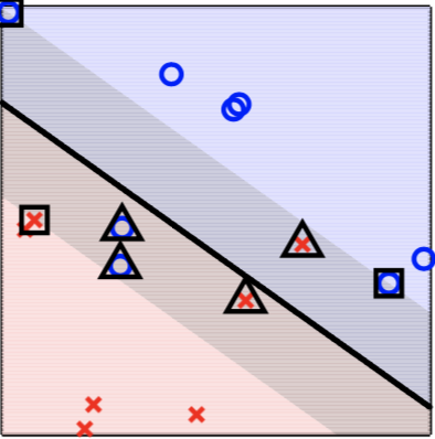
- when $\alpha_n=0$, then $\xi_n=0$. The sample is non support vector which should be away from the boundary.
- when $0<\alpha_n<C$, then $\xi_n=0$. The sample is a free support vector located on the boundary. (square in figure)
- when $\alpha_n=C$, then $\xi_n>0$ describes violation amount. The sample violates the boundary. (triangle in figure)
At the same time, we find that $\xi_n=1-y_n(\boldsymbol w^\text T\boldsymbol x_n+b)$ if $\boldsymbol x_n$ violates the margin and else $\xi_n=0$. In a brief form, we have
\[\xi_n=\max\left(1-y_n(\boldsymbol w^\text T\boldsymbol x_n+b),0\right) \tag{9.39}\]according to this formula, we can rewrite our objective in $(9.32)$ as follows:
\[\min_{b,\boldsymbol w} \ \ \frac{1}{2}\boldsymbol w^\text T\boldsymbol w+C \cdot \sum_{n=1}^N\max\left(1-y_n(\boldsymbol w^\text T\boldsymbol x_n+b),0\right) \tag{9.40}\]Consider the first item in this formula as L-2 regularizer and the second item describes the degree of error, then the soft-margin SVM can be classified as a kind of a unique form of regularization.
Kernel Logistic Regression
Kernel tricks help us save expense of calculating in high dimension space, it can also be applied into logistic regression like a ‘two-level learning’.
With feature transformation $\boldsymbol\Phi(\boldsymbol x)$, the optimal hypothesis of logistic regression is written as
\[g(\boldsymbol x) = \sigma(\boldsymbol w^\text T\boldsymbol\Phi(\boldsymbol x)+b) \tag{9.41}\]according to previous derivation, we have
\[\boldsymbol w^\text T\boldsymbol\Phi(\boldsymbol x)+b=\sum_{n=1}^N\alpha_ny_nK_{\boldsymbol\Phi}(\boldsymbol x_n,\boldsymbol x)+y_s-\sum_{n=1}^N\alpha_ny_nK_{\boldsymbol\Phi}(\boldsymbol x_n,\boldsymbol x_s) \tag{9.42}\]view $\boldsymbol w^\text T\boldsymbol\Phi(\boldsymbol x)+b$ as a special transform, recorded as $\Phi_\text{SVM}(\boldsymbol x)$, which can easily calculted with kernel tricks, then $g$ becomes
\[g(\boldsymbol x)=\sigma\left(A\cdot\Phi_\text{SVM}(\boldsymbol x)+B\right) \tag{9.43}\]where $A$ describes scaling and $B$ describes shifting, then the optimization goal in logistic regression becomes
\[\min_{A,B} \ \frac{1}{N}\sum_{n=1}^N\ln\left(1+\exp\left(-y_n(A\cdot\Phi_\text{SVM}(\boldsymbol x)+B\right)\right) \tag{9.44}\]then the problem has reduced to a 1st-dim logistic regression with only two variables.
This method finding a transform $\Phi_\text{SVM}(\boldsymbol x)$ in a high space and return a scalar value, next we try to do exact logistic regression in the high space with kernel. Consider L-2 regularized logistic regression, the optimization goal is
\[\min_{\boldsymbol w} \ \frac{1}{N}\sum_{n=1}^N\ln(1+ \exp (-y_n\boldsymbol w^{\text T}\boldsymbol x_n)) + \frac{\lambda}{N}\boldsymbol w^\text T\boldsymbol w \tag{9.45}\]from which we can ensure the final $\boldsymbol w$ is the linear combination of $\boldsymbol x_n$, and we can further prove it established for each L-2 regularized linear model
\[\min_{\boldsymbol w} \ \frac{\lambda}{N}\boldsymbol w^\text T\boldsymbol w+\frac{1}{N}\sum_{n=1}^N\text{err}(y_n, \boldsymbol w^\text T\boldsymbol x) \tag{9.46}\]the optimal $\boldsymbol w$ can be written as $\boldsymbol w_\ast=\sum_{n=1}^N\beta_n\boldsymbol x_n$. Assume we have a optimal $\boldsymbol w_\ast$ violates this equality, and $\boldsymbol w_\ast=\boldsymbol w_\bot+\boldsymbol w_\Vert$, where $\boldsymbol w_\bot \in \text{ span}(\boldsymbol x_n)$ and $\boldsymbol w_\Vert \bot \text{ span}(\boldsymbol x_n)$. then we have
\[\text{err}(y_n, \boldsymbol w_*^\text T\boldsymbol x)=\text{err}(y_n, (\boldsymbol w_\bot+\boldsymbol w_\Vert)^\text T\boldsymbol x) = \text{err}(y_n, \boldsymbol w_\Vert^\text T\boldsymbol x) \tag{9.47}\]another hand
\[\begin{split} \boldsymbol w_*^\text T\boldsymbol w_* &= \boldsymbol w_\bot^\text T\boldsymbol w_\bot + 2\boldsymbol w_\bot^\text T\boldsymbol w_\Vert + \boldsymbol w_\Vert^\text T\boldsymbol w_\Vert \\[1em] &= \boldsymbol w_\bot^\text T\boldsymbol w_\bot + \boldsymbol w_\Vert^\text T\boldsymbol w_\Vert \\[1em] &\ge \boldsymbol w_\Vert^\text T\boldsymbol w_\Vert \end{split} \tag{9.48}\]so we have a better $\boldsymbol w_\Vert$ more optimal than $\boldsymbol w_*$ which is a contradiction.
With this condition, substitute the optimal $\boldsymbol w_*=\sum_{i=1}^N\beta_i\boldsymbol x_i$ into the goal function, we have
\[\begin{split} \boldsymbol w^\text T\boldsymbol x_n &= \sum_{i=1}^N\beta_i\boldsymbol x_i^\text T\boldsymbol x_n = \sum_{n=1}^N\beta_iK(\boldsymbol x_i,\boldsymbol x_n) \\[1em] \boldsymbol w^\text T\boldsymbol w &= \sum_{i=1}^N\beta_i\boldsymbol x_i^\text T \cdot \sum_{i=1}^N\beta_i\boldsymbol x_i \\[1em] &= \sum_{i=1}^N\sum_{j=1}^N\beta_i\beta_jK(\boldsymbol x_i,\boldsymbol x_j) \end{split} \tag{9.49}\]then the problem becomes finding a optimal $\boldsymbol\beta$ instead of $\boldsymbol w$
\[\min_{\boldsymbol \beta} \ \frac{1}{N}\sum_{n=1}^N\ln\left(1+ \exp \left(-y_n\sum_{n=1}^N\beta_iK(\boldsymbol x_i,\boldsymbol x_n)\right)\right) + \frac{\lambda}{N}\sum_{i=1}^N\sum_{j=1}^N\beta_i\beta_jK(\boldsymbol x_i,\boldsymbol x_j)\tag{9.50}\]this form is called Kernel Logistic Regression, easily find it is quite similar with SVM.
Support Vector Regression
In general rigde regression, we measure the error in training dataset with square error $(y_n-\boldsymbol w^\text T\boldsymbol x_n)^2$, according to our derivation above, it can be rewritten with kernel as $\left(y_n-\sum_{i=1}^N\beta_iK(\boldsymbol x_i,\boldsymbol x_n)\right)^2$. Then our optimization goal is
\[\min_{\boldsymbol \beta} \ \frac{1}{N}\sum_{n=1}^N\left(y_n-\sum_{i=1}^N\beta_iK(\boldsymbol x_i,\boldsymbol x_n)\right)^2 + \frac{\lambda}{N}\sum_{i=1}^N\sum_{j=1}^N\beta_i\beta_jK(\boldsymbol x_i,\boldsymbol x_j)\tag{9.51}\]this complicated formula can be simplified with matrix form as follows:
\[\begin{split} &\min_{\boldsymbol\beta} \ \frac{1}{N}\Vert\boldsymbol y-\boldsymbol {K\beta}\Vert + \frac{\lambda}{N}\boldsymbol\beta^\text T\boldsymbol{K\beta} \\[1em] =& \min_{\boldsymbol\beta} \frac{1}{N}\left(\boldsymbol\beta^\text T\boldsymbol K^\text T\boldsymbol{K\beta}-2\boldsymbol\beta^\text T\boldsymbol K^\text T\boldsymbol y + \boldsymbol y^\text T\boldsymbol y \right) + \frac{\lambda}{N}\boldsymbol\beta^\text T\boldsymbol{K\beta} \end{split} \tag{9.52}\]record this objective as $E_\text{aug}$ and then differentiate $\boldsymbol\beta$, we have
\[\begin{split} \nabla_{\boldsymbol\beta}E_\text{aug} &= \frac{2}{N}\left(\lambda\boldsymbol {K\beta}+\boldsymbol K^\text T\boldsymbol {K\beta}-\boldsymbol K^\text T\boldsymbol y\right) \\[1em] &= \frac{2}{N}\boldsymbol K^\text T\left((\lambda\boldsymbol I+\boldsymbol K)\boldsymbol\beta-\boldsymbol y\right) \end{split} \tag{9.53}\]set $\nabla_{\boldsymbol\beta}E_\text{aug}=0$, we have one analytic solution
\[\boldsymbol\beta=(\lambda\boldsymbol I+\boldsymbol K)^{-1}\boldsymbol y \tag{9.54}\]this inverse matrix always exists because we have $\lambda>0$ and $\boldsymbol K$ is positive semi-definite. Complexity of train with kernel regression is $O(N^3)$, which is quite high for big data, and in that case, linear regression may be a good alternatives.
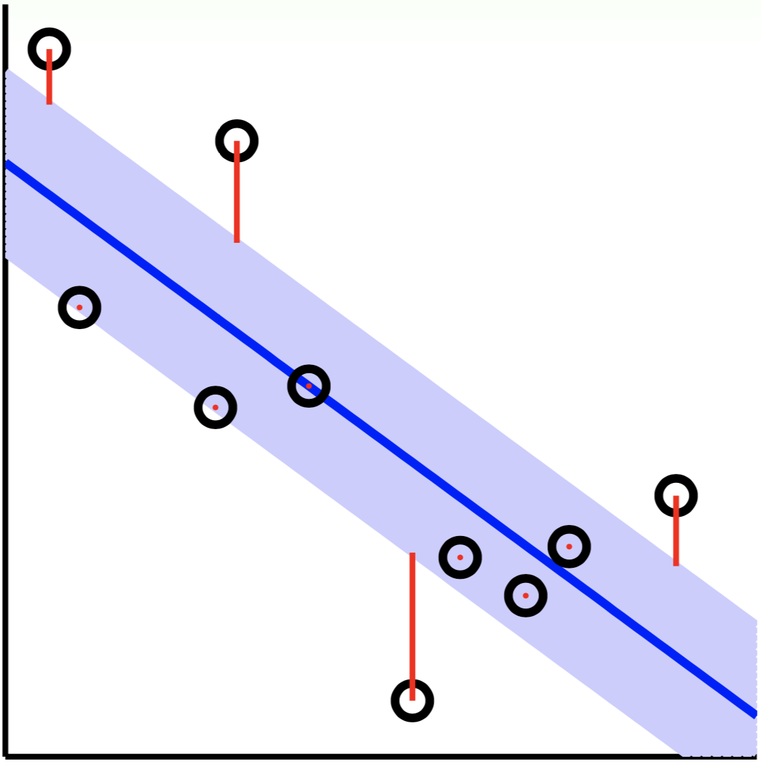
Similar to soft-margin SVM, we consider a special ‘tube’ regression

as shown in above image, points in the tube is regarded as no error while points outside the tube have a error measured by distance to tube. That is
\[\text{err}(y,\hat y)= \begin{cases} 0 & |\hat y-y| \le \epsilon \\[1em] |\hat y-y|-\epsilon & |\hat y-y| > \epsilon \end{cases} \tag{9.55}\]where $\hat y=\boldsymbol w^\text T\boldsymbol x_n+b$, in general we have
\[\text{err}(y, \hat y)= \max(0,|\hat y-y|-\epsilon) \tag{9.56}\]this form of error is called $\epsilon$-insentive Error with $\epsilon>0$. Then our optimization goal is
\[\min_{b,\boldsymbol w} \ C\sum_{n=1}^N\max(0, \vert\hat y_n-y_n\vert - \epsilon)+\frac{1}{2}\boldsymbol w^\text T\boldsymbol w \tag{9.57}\]the $\max$ function is non-differentiable in some point, we introduce a slack variable $\xi_n = \max(0, \vert \hat{y}_n - y_n \vert - \epsilon)$ similar to soft-margin SVM, and rewrite $(9.57)$
\[\begin{split} \min_{b,\boldsymbol w,\boldsymbol\xi} \ &C\sum_{n=1}^N\xi_n+\frac{1}{2}\boldsymbol w^\text T\boldsymbol w \\[1em] \text{s.t.} \ &|\hat y_n-y_n| \le \epsilon+\xi_n \\[1em] & \xi_n \ge 0 \end{split} \tag{9.58}\]in this formula, when $\vert\hat y_n-y_n\vert-\epsilon \le 0$, in order to minimize the objective, it should have $\xi_n=0$, and when $\vert\hat y_n-y_n\vert - \epsilon > 0$, then $\xi_n \ge \vert\hat y_n-y_n\vert-\epsilon$ according to the first constraint, to minimize the objective, we have $\xi_n = \vert\hat y_n-y_n\vert-\epsilon$. This shows that introducing this variable is reasonable. Further, remove absolute value and transform the constraint into linear form
\[\begin{split} \min_{b,\boldsymbol w,\boldsymbol\xi^<,\boldsymbol\xi^>} \ &C\sum_{n=1}^N(\xi_n^<+\xi_n^>)+\frac{1}{2}\boldsymbol w^\text T\boldsymbol w \\[1em] \text{s.t.} \ &\boldsymbol w^\text T\boldsymbol x_n+b-y_n \le \epsilon+\xi_n^> \\[1em] &\boldsymbol w^\text T\boldsymbol x_n+b-y_n \ge -\epsilon-\xi_n^< \\[1em] & \xi_n^< \ge 0, \ \xi_n^> \ge 0 \end{split} \tag{9.59}\]where $\xi_n^<$ is the lower tube violations while $\xi_n^>$ is the upper tube violations. Introduce Lagrange multipliers $\alpha^<_n$ and $\alpha^>_n$, then do some calculations as before, we can have some of the KKT conditions:
\[\begin{align} \boldsymbol w &= \sum_{n=1}^N(\alpha_n^<-\alpha_n^>)\boldsymbol x_n \tag{9.60} \\[1em] 0 &= \sum_{n=1}^N(\alpha_n^<-\alpha_n^>) \tag{9.61} \\[1em] 0 &= \alpha_n^<(\boldsymbol w^\text T\boldsymbol x_n+b-y_n+\epsilon+\xi_n^<) \tag{9.62} \\[1em] 0 &= \alpha_n^>(\boldsymbol w^\text T\boldsymbol x_n+b-y_n-\epsilon-\xi_n^>) \tag{9.63} \\[1em] \end{align}\]similarly, we can get the dual probblem of SVR, which can be solved with QP computing program. According to formula $(9.62)$ and $(9.63)$, we have the following two situations:
For points within tube, we have
\[\begin{split} &|\boldsymbol w^\text T\boldsymbol x_n+b-y_n| \le \epsilon \\[1em] \Rightarrow \ & \xi_n^<=0, \ \xi_n^>=0 \\[1em] \Rightarrow \ & \boldsymbol w^\text T\boldsymbol x_n+b-y_n+\epsilon+\xi_n^< \ne 0, \ \boldsymbol w^\text T\boldsymbol x_n+b-y_n-\epsilon-\xi_n^> \ne 0 \\[1em] \Rightarrow \ &\alpha_n^<=0, \ \alpha_n^>=0 \end{split} \tag{9.64}\]clearly, these points make no contribution to the final $\boldsymbol w$.
For points outside tube, which are support vectors in this model, we can calculate $\boldsymbol w$ and $b$ through these points.
