Factors Leading to Overfitting
- Number of samples is too small
- Too much noise
- Excessively complicated model
Weight-decay Regularization
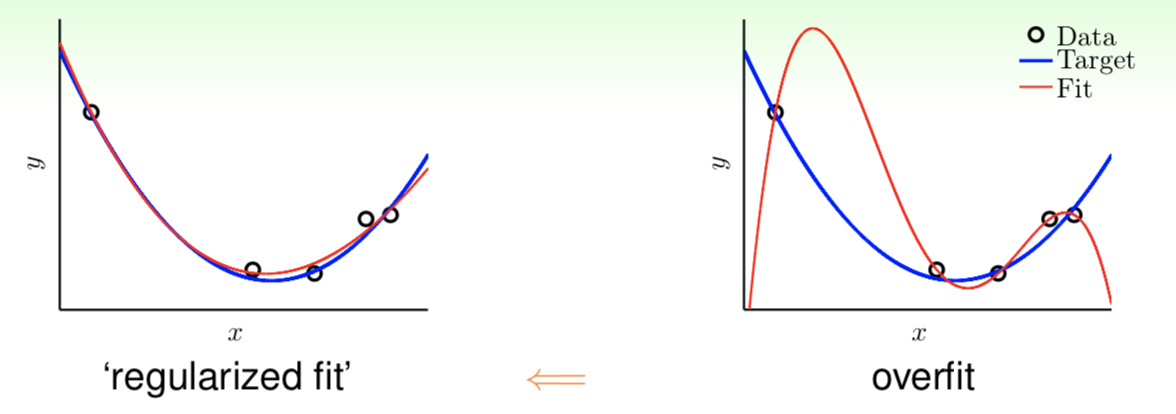
Firstly, look at a typical example of overfitting:

As shown, a high-order polynomial (such as 10th-order) performed not very well when dataset is not large enough. One of our ideas to reduce overfitting is ‘stepping back’ from $\mathcal H_{10}$ to $\mathcal H_2$. For convenience, we denote $\tilde {\boldsymbol w}$ as $\boldsymbol w$. For $x \in \mathbb R$, we have
\[\begin{split} \mathcal H_{10}&:w_0+w_1x+w_2x^2+w_3x^3\cdots+w_{10}x \\[1em] \mathcal H_2&:w_0+w_1x+w_2x \end{split} \tag{8.1}\]obviously, $\mathcal H_{10}=\mathcal H_2$ when $w_3=w_4=\cdots=w_{10}=0$. Make this constraint a little looser, we set
\[\mathcal H_2'=\{\ \boldsymbol w\in \mathbb R^{10+1}\ \ \text{while more than } 8 \text{ of } w_q=0\} \tag{8.2}\]then regression with $\mathcal H_2’$ is
\[\begin{split} \min_{\boldsymbol w\in \mathbb R^{10+1}}& \ E_{\text{in}}(\boldsymbol w) \\[1em] \text{s.t.}& \ \sum_{q=0}^{10}[\![w_q\ne0]\!] \le 3 \end{split} \tag{8.3}\]However, bad news is that optimization of this formula is NP-hard to solve, we have to replace it with a softer constraint as follows:
\[\mathcal H_2'=\{\ \boldsymbol w\in \mathbb R^{10+1}\ \ \text{while } \Vert\boldsymbol w\Vert^2 \le C \} \tag{8.4}\]regression is
\[\begin{split} \min_{\boldsymbol w\in \mathbb R^{10+1}}& \ E_{\text{in}}(\boldsymbol w) \\[1em] \text{s.t.}& \ \sum_{q=0}^{10}w_q^2 \le C \end{split} \tag{8.5}\]Similar to linear regression, we record the in-sample error as$E_{\text{in}}(\boldsymbol w)=\frac{1}{N}\Vert\boldsymbol {Zw}-\boldsymbol y\Vert^2$. Consider the general form when feature dimension is $Q$, we have optimization goal:
\[\begin{split} \min_{\boldsymbol w\in \mathbb R^{Q+1}}& \ \frac{1}{N}(\boldsymbol {Zw}-\boldsymbol y)^{\text T}(\boldsymbol {Zw}-\boldsymbol y) \\[1em] \text{s.t.}& \ \boldsymbol w^{\text T}\boldsymbol w \le C \end{split} \tag{8.6}\]we call this model Regularized Hypothesis, and the optimal weight vector of which is recorded as $\boldsymbol w_{\text{REG}}$.
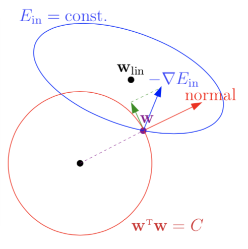
Next we try to solve this optimization problem. Look at the image below

in non-constraint optimization, we search in the opposite direction of the gradient to find the optimal solution. However, feasible $\boldsymbol w$ here must be within a radius-$\sqrt C$ hypersphere and in most cases the optimal solution will be at the edge of it. Suppose there already have a $\boldsymbol w$ at the edge, then we can judge whether it is the optimal by judging whether it can proceed in the opposite direction of gradient under constraint. And we can see from the figure clearly that only if $\boldsymbol w$ walk along the tangential direction of the hypersphere can it stays within the hypersphere. Focus on the green vector in above figure, if -$\nabla E_{\text{in}}(\boldsymbol w)$ has a component in the tangential direction of the hypersphere, we can get a better $\boldsymbol w$ by the direction of this component. That is, the $\boldsymbol w$ is optimal only when $\nabla E_{\text{in}}(\boldsymbol w)$ is in the same direction with $\boldsymbol w$, the normal vector of the hypersphere. So we try to find Lagrange multiplier $\lambda>0$ and $\boldsymbol w_\text{REG}$ such that:
\[\nabla E_{\text{in}}(\boldsymbol w_\text{REG})+\frac{2\lambda}{N}\boldsymbol w_\text{REG}=\boldsymbol 0 \tag{8.7}\]where $\frac{2\lambda}{N}$ is set in order to facilitate subsequent calculation. Similar to linear regression, we rewrite $(8.7)$ as follows:
\[\begin{split} &\frac{2}{N}(\boldsymbol {Z}^\text T\boldsymbol {Z}\boldsymbol w_\text{REG}-\boldsymbol {Z}^\text T\boldsymbol y)+\frac{2\lambda}{N}\boldsymbol w_\text{REG}&=\boldsymbol 0 \\[1em] &\Rightarrow (\boldsymbol {Z}^\text T\boldsymbol {Z}\boldsymbol w_\text{REG}-\boldsymbol {Z}^\text T\boldsymbol y)+\lambda\boldsymbol w_\text{REG}&=\boldsymbol 0 \end{split} \tag{8.8}\]Solve this equation, we have
\[\boldsymbol w_\text{REG}=(\boldsymbol {Z}^\text T\boldsymbol {Z}+\lambda\boldsymbol I)^{-1}\boldsymbol {Z}^\text T\boldsymbol y \tag{8.9}\]which we called Ridge Regresson in statistics. It’s easy to prove $\boldsymbol {Z}^\text T\boldsymbol {Z}+\lambda\boldsymbol I$ is positive-definite when $\lambda>0$.
Regard $(8.7)$ as the derivative of $E_\text{in}(\boldsymbol w)+\frac{\lambda}{N}\boldsymbol w^\text T\boldsymbol w$, which is called Augmented Error, recorded as $E_\text{aug}(\boldsymbol w)$, and where $\boldsymbol w^\text T\boldsymbol w$ is called Regularizer. This kind of regularization preferring a shorter $\boldsymbol w$ is called Weight-decay Regularization. Lagrange multiplier $\lambda$ is related to $C$, represents the strength of constraint, in this opinion, we think that $\lambda=0$ is also acceptable because it represents a regression without restraint. We can get different results using different $\lambda$ as follows:

By the way, if we limit each component of $\boldsymbol x$ within scope of $[-1,1]$, the $n$th-oreder polynomial would be so little that penalty $\lambda$ seems too heavy. In this case, we can replace simple polynomials such as $x,x^2,x^3,…x^n$ with Legendre Polynomials. It may have a better fitting result.
Connection to VC Theory
Look at this problem from the perspective of VC theory, we have
\[\begin{gather} E_\text{aug}(\boldsymbol w) = &E_\text{in}(\boldsymbol w)+\frac{\lambda}{N}\boldsymbol w^\text T\boldsymbol w \tag{8.10} \\[1em] E_\text{out}(\boldsymbol w) \le &E_\text{in}(\boldsymbol w)+\Omega(\mathcal H) \tag{8.11} \end{gather}\]where $\boldsymbol w^\text T\boldsymbol w$ represents complexity of a single hypothesis and $\Omega(\mathcal H)$ represents complexity of whole hypothesis set. When constraint $C$ introduced, effective hypotheses have been grately reduced. Record effective VC dimension of hypothesis set as $d_\text{EFF}(\mathcal {H,A} )$, where $\mathcal A$ represents regularized algorithm under constraint. When $\lambda>0$, we have:
\[d_\text{EFF}(\mathcal{H,A}) \le d_\text{VC} \tag{8.12}\]As $\lambda$ increased, more $\boldsymbol w$ will be discarded and $d_\text{EFF}$ will be lower.
