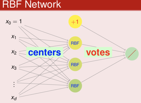
RBF Network Learning
Firstly we consider the Gaussian SVM which map our data to a infinite-dimensional space
\[g_\text{SVM}(\boldsymbol x) = \text{sign}\left(\sum_\text{SV}\alpha_ny_n\exp(-\gamma\Vert\boldsymbol x-\boldsymbol x_n\Vert^2)+b\right) \tag{12.1}\]here Gaussian kernel is also called Radial Basis Function(RBF) and radial means this model only depends on distance between $\boldsymbol x$ and ‘center’ $\boldsymbol x_n$.
Let $g_n(\boldsymbol x)=y_n\exp(-\gamma\Vert\boldsymbol x-\boldsymbol x_n\Vert^2)$, then $(12.1)$ is rewritten as
\[g_\text{SVM}(\boldsymbol x) = \text{sign}\left(\sum_\text{SV}\alpha_ng_n(\boldsymbol x)+b\right) \tag{12.2}\]it can be referred as a neural network whose hidden layer consists of those ‘center’ points and output layer is simple linear aggregation

in a general form, RBF network hypothesis is
\[h(\boldsymbol x)=\text{Output}\left(\sum_\text{m=1}^M\beta_m\text{RBF}(\boldsymbol x, \boldsymbol \mu_m)+b\right) \tag{12.3}\]and the key variables in this model is each center $\boldsymbol\mu_m$, and in SVM that is the support vectors.
In order to determine the center $\boldsymbol\mu_m$, we firstly consider a simple situation called full RBF network, where we consider all the points in the dataset as the center, that is we set $M$ simply equal to $N$. And we know the Gaussian function decrease at a very fast rate, so the final summation tends to be decided by the nearest neighbor $\boldsymbol\mu_m$ of the input $\boldsymbol x$, that is
\[g_\text{nbor}(\boldsymbol x)=y_m \ \ \ \ \ \text{such that } \boldsymbol x \text{ closest to } \boldsymbol x_m \tag{12.4}\]further, we can also choose $k$ neighbors to aggregate which is called $k$ nearest neighbor.
Next we try to use squared error regression to calculate the optimal $\beta_m$ in full RBF Network instead of the lazy method mentioned above. Similar to linear regression, we rewrite the hypothesis as follows
\[h(\boldsymbol x)=\sum_\text{n=1}^n\beta_n\text{RBF}(\boldsymbol x, \boldsymbol x_n) \tag{12.5}\]record $\boldsymbol z_n = (\text{RBF}(\boldsymbol x_n, \boldsymbol x_1),\text{RBF}(\boldsymbol x,_n \boldsymbol x_2),…,\text{RBF}(\boldsymbol x_n, \boldsymbol x_N))^\text T$, and according to the derivation in linear regression, we can similarly get the optimal $\boldsymbol\beta$
\[\boldsymbol \beta =(\boldsymbol Z^\text T\boldsymbol Z)^{-1}\boldsymbol Z^\text T\boldsymbol y \tag{12.6}\]another hand, here $\boldsymbol Z$ is a symmetric square matrix, then $(12.6)$ can be reduced to
\[\boldsymbol \beta=\boldsymbol Z^{-1}\boldsymbol y \tag{12.7}\]and use this $\boldsymbol \beta$ we find the inner error rate is $0$, obviously when we apply this model to action, it may cause serious overfit. So we commonly use ridge regression for $\boldsymbol \beta$ instead.
\[\boldsymbol \beta =(\boldsymbol Z^\text T\boldsymbol Z+\lambda\boldsymbol I)^{-1}\boldsymbol Z^\text T\boldsymbol y \tag{12.8}\]Another way to regularize is choosing some points in the whole set as prototypes, and then consider these points as centers $\boldsymbol \mu_m$.
k-Means Algorithm
Next we try to cluster with the prototype $\boldsymbol\mu_m$, divide the whole dataset into $M$ disjoint sets $S_1, S_2, … , S_M$ and choose $\boldsymbol\mu_m$ for each $S_m$. For each $\boldsymbol x_i, \boldsymbol x_j$ both belong to $S_m$, we hope that $\boldsymbol \mu_m \approx \boldsymbol x_i \approx \boldsymbol x_j$.The squared error is
\[E_\text{in}(S_1,S_2,...,S_M;\boldsymbol\mu_1,\boldsymbol\mu_2,...,\boldsymbol\mu_M)=\frac{1}{N}\sum_{n=1}^N\sum_{m=1}^M[\![\boldsymbol x_n \in S_m]\!]\Vert\boldsymbol x_n-\boldsymbol \mu_m\Vert^2 \tag{12.9}\]this problem is hard to optimize, we consider $\lbrace S_m\rbrace_{m=1}^M, \lbrace\boldsymbol \mu_m\rbrace_{m=1}^M$ as two sets of variables and then optimize them respectively. When $S_1,S_2,…,S_M$ is fixed, we derivative $E_\text{in}$ on $\boldsymbol\mu_m$
\[\begin{split} \nabla_{\boldsymbol\mu_m}E_\text{in} &= -2\sum_{n=1}^N[\![\boldsymbol x_n \in S_m]\!](\boldsymbol x_n-\boldsymbol\mu_m) \\[1em] &=-2\left(\sum_{\boldsymbol x_n \in S_m}\boldsymbol x_n-|S_m|\boldsymbol \mu_m\right) \end{split} \tag{12.10}\]then set $\nabla_{\boldsymbol\mu_m}E_\text{in}=0$, we will find the optimal $\boldsymbol \mu_m$ is just the average of $\boldsymbol x_n$ within $S_m$. When $\boldsymbol\mu_1,\boldsymbol\mu_2,…,\boldsymbol\mu_M$ is fixed, we optimize $S_m$ by divide each $\boldsymbol x_n$ into the cluster with the closest $\boldsymbol\mu_m$.
Finally, we get the $k$-Means Algorithm, in which we first choose $k$ $\boldsymbol x_n$ randomly as $\boldsymbol\mu_1,\boldsymbol\mu_2,…\boldsymbol\mu_k$ and then keep optimizing $S_1,S_2,…,S_k$ and $\boldsymbol\mu_1,\boldsymbol\mu_2,…,\boldsymbol\mu_k$ until converge.
