For $\boldsymbol{x}=(x_1,x_2,…,x_d)$, compute a weighted ‘score’. Judging as positive if $\sum_{i=1}^dw_ix_i>\text{threshold}$ while judging as negative if $\sum_{i=1}^dw_ix_i<\text{threshold}$.
Using $\mathcal{Y}:\lbrace+1,-1\rbrace$ represent two classification results, linear formula $h\in\mathcal{H}$ are
\[h(\boldsymbol{x})=\text{sign}\left(\left(\sum_{i=1}^dw_ix_i\right)-\text{threshold}\right) \tag{3.1}\]In $(3.1)$, set $-\text{threshold}=w_0$ and $+1=x_0$. Then
\[\begin{split} h(\boldsymbol{x}) &=\text{sign}\left(\sum_{i=0}^dw_ix_i\right) \\ &=\text{sign}\left(\boldsymbol{w}^\text{T}\boldsymbol{x}\right) \end{split} \tag{3.2}\]In order to find a best straight line to completely separate all the positive and negative examples on the plane, we can use the idea of ‘point-by-point correction’. First, take a straight line on the plane to see which points are classified incorrectly. Then start to correct the error point in the first attempt, that is, change the position of the line, so that the error point becomes classified correctly. Then, the second, third, and so on until all the error classification points are separated correctly in a straight line.
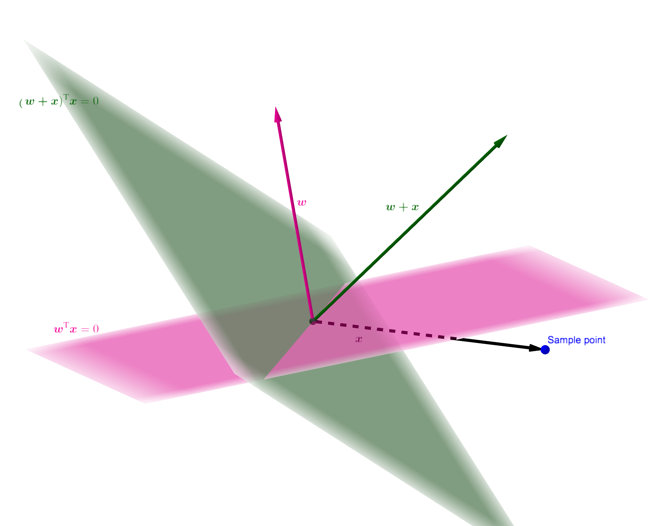
Next we introduce the perceptron learning algorithm (PLA). First, randomly select a line to classify. Then find the first point of the classification error. If this point represents a positive example but misclassified as a negative example, that is $\boldsymbol w_t^\mathrm{T} \boldsymbol x_{n(t)} < 0$, which means the angle between $\boldsymbol w_t$ and $\boldsymbol x_{n(t)}$ is over $\frac{\pi}{2}$, and where $\boldsymbol w_t$ is the normal vector of the line. Therefore, $\boldsymbol x_{n(t)}$ is mis-divided on the lower side of the line (relative to the normal vector, the direction of the normal vector is the side where the positive class is located). The correction method is to make $\boldsymbol w_{t}$ and $\boldsymbol x_{n(t)}$ less than $\frac{\pi}{2}$. A common way to do this is set $\boldsymbol w_{t+1} \gets \boldsymbol w_t + \boldsymbol x_{n(t)}$.
Similarly, if a point is misclassified as negative example, that means $\boldsymbol w_t$ and $\boldsymbol x_{n(t)}$are less than $\frac{\pi}{2}$, where $\boldsymbol w_t$ is the normal vector of the line. So, $\boldsymbol x_{n(t)}$ is misclassified in the line on the upper side, the correction is to make $\boldsymbol w_t$ and $\boldsymbol x_{n(t)}$ greater than $\frac{\pi}{2}$ with $\boldsymbol w_{t+1} \gets \boldsymbol w_t-\boldsymbol x_{n(t)}$.
In summary, when an error point found, we have iterative formula of PLA
\[\boldsymbol w_{t+1} \gets \boldsymbol w_t+y_{n(t)}\boldsymbol x_{n(t)} \tag{3.3}\]
PLA works well in 3D or even higher space, as shown in the figure above, the sample point is located on the lower side of plane determined by $\boldsymbol w$ but it located on the upper side of plane after modification.
According to the method mentioned above, PLA keeps finding error point and iterating. It is important to note that in each iteration it may cause the previously classified point to become a wrong point. But it does’t matter because constant iteration will eventually classify all points correctly (the premise is linear separability).
In practice, we can check each point one by one, and correct the wrong point immediately. Keep iteration until all points are classified correctly. At this time, complexity of each iteration is $O(1)$.
