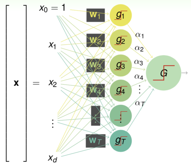
Neural Network is a classic algorithm originated from perceptron. Linearly combine various perceptrons such as the figure

the final hypothesis $G$ is
\[G(\boldsymbol x)=\text{sign}\left(\sum_{t=1}^T\alpha_t\underbrace{\text{sign}(\boldsymbol w^\text T_t\boldsymbol x)}_{g_t(\boldsymbol x)}\right) \tag{11.1}\]it is a neural network of two layers, and $\boldsymbol\alpha$ and $\boldsymbol w_t$ is weights of each layer. Through adding more layers wa can make the model more powerful. Another hand, we replace $\text{sign}$ function with $\tanh$ function which has good mathematical properties.
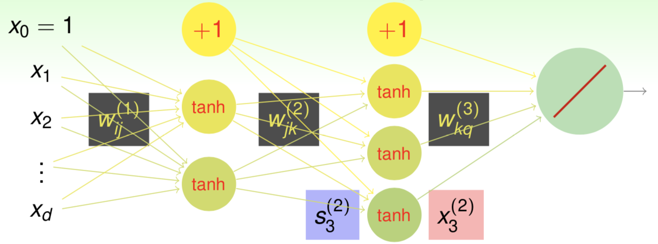
\[\tanh(x) = \frac{\exp(x)-\exp(-x)}{\exp(x)+\exp(-x)} \tag{11.2}\]Consider a more complex neural network with $L$ layers

the input $\boldsymbol x$ can be regarded as the $0$-th layer, then record numbers of nodes in each layer as $d^{(0)}, d^{(1)}, … , d^{(L)}$, and $w_{ij}^{(\ell)}$ is weight in $\ell$-th layer from $i$-th node in $(\ell-1)$-th layer to $j$-th node in $\ell$-th layer, $s_j^{(\ell)}$ is score of $j$-th node in $\ell$-th layer, $x_i^{(\ell)}$ is transformed input of $i$-th node in $\ell$-th layer.
\[\begin{align} s_j^{(\ell)} &= \sum_{i=0}^{d^(\ell-1)}w_{ij}^{(\ell)}x_i^{(\ell-1)} \tag{11.3} \\[1em] x_j^{(\ell)} &= \begin{cases} \tanh(s_j^{(\ell)}) & \ell < L \\[1em] s_j^{(l)} & \ell=L \end{cases} \tag{11.4} \end{align}\]Next we try to learn the optimal weight. Firstly consider the output layer, error of $\boldsymbol x_n$ is
\[\begin{split} E_n &= \left(y_n-s_1^{(L)}\right)^2 \\[1em] &= \left(y_n-\sum_{i=0}^{d^{(L-1)}}w_{i1}^{(L)}x_i^{(L-1)}\right)^2 \end{split} \tag{11.5}\]we have
\[\begin{split} \frac{\partial E_n}{\partial w_{i1}^{(L)}} &= \frac{\partial E_n}{\partial s_1^{(L)}} \cdot \frac{\partial s_1^{(L)}}{\partial w_{i1}^{(L)}} \\[1em] &= -2\left(y_n-s_1^{(L)}\right) \cdot x_i^{(L-1)} \end{split} \tag{11.6}\]record $\delta_1^{(L)}=-2\left(y_n-s_1^{(L)}\right)$, similarly we can get derivation in general $\ell$-th layer
\[\begin{split} \frac{\partial E_n}{\partial w_{ij}^{(\ell)}} &= \frac{\partial E_n}{\partial s_j^{(\ell)}} \cdot \frac{\partial s_j^{(\ell)}}{\partial w_{ij}^{(\ell)}} \\[1em] &= \delta_j^{(\ell)} \cdot x_i^{(\ell-1)} \end{split} \tag{11.7}\]next we try to get $\delta_j^{(\ell)}$. To get $E_n$ from $s_j^{(\ell)}$, we have the following process
\[s_j^{(\ell)} \mathop{\Longrightarrow}^{\tanh} x_j^{(\ell)} \mathop{\Longrightarrow}^{w_{jk}^{(\ell+1)}} \left( \begin{array}{ccc} s_1^{(\ell+1)} \\[0.5em] \vdots \\[0.5em] s_k^{(\ell+1)} \\[0.5em] \vdots \end{array} \right) \Longrightarrow \cdots \Longrightarrow E_n \tag{11.8}\]use chain rule to get the derivation
\[\begin{split} \delta_j^{(\ell)} &= \frac{\partial E_n}{\partial s_j^{(\ell)}} = \sum_{k=1}^{d^{(\ell+1)}} \frac{\partial E_n}{\partial s_k^{(\ell+1)}} \cdot \frac{\partial s_k^{(\ell+1)}} {\partial x_j^{(\ell)}} \cdot \frac{\partial x_j^{(\ell)}}{\partial s_j^{(\ell)}} \\[1em] &= \sum_{k=1}^{d^{(\ell+1)}} \delta_k^{(\ell+1)} \cdot w_{jk}^{(\ell+1)} \cdot \tanh'\left(s_j^{(\ell)}\right) \end{split} \tag{11.9}\]from $(11.9)$ we get the recursive formula of $\delta^{(\ell)}$ and $\delta^{(\ell+1)}$, and based on it we have Backpropagation Algorithm.
Algorithm
Initialize all weights $w_{ij}^{(\ell)}$
for $t=0,1,…,T$
- stochastic: randomly pick $n \in {1,2,…,N}$
- forward: compute all $x_i^{(\ell)}$ with $\boldsymbol x^{(0)}=\boldsymbol x_n$
- backward: compute all $\delta_j^{(\ell)}$ subject to $\boldsymbol x^{(0)}=\boldsymbol x_n$
- gradient descent: $w_{ij}^{(\ell)} \gets w_{ij}^{(\ell)}-\eta\delta_j^{(\ell)}x_i^{(\ell-1)}$
return
