Components of Machine Learning
- Input (sample vector): $\boldsymbol{x}\in\mathcal{X}$
- Output: $y\in\mathcal{Y}$
- Unknown pattern to be leared (target function): $f:\mathcal{X}\to\mathcal{Y}$
- Data set (training examples): $\mathcal{D}=\lbrace(\boldsymbol{x_i},y_i)\rbrace_{i=1}^N$
- Hypotheses set (set of candidate formula): $\mathcal{H}=\lbrace h\vert h:\mathcal{X}\to \mathcal{Y}\rbrace$
- Learning algorithm: $\mathcal A$
- Final hypothesis (learned formula with hopefully good performance): $g:\mathcal{X}\to\mathcal{Y}$
Computational Theory
Growth Function
Record the prediction error rate of final hypothesis $g$ in the sample set and the whole input space as $E_{\text{in}}(g)$ and $E_{\text{out}}(g)$ respectively. Then we have two major problem of machine learning:
- $E_{\text{in}}(g) \approx E_{\text{out}}(g)$
- $E_{\text{in}}(g)$ is small enough
When each $h\in\mathcal H$ is independently distributed, from Hoeffding inequality we have
\[P[\![|E_{\text{in}}(g) - E_{\text{out}}(g) |>\epsilon]\!]\le2M\cdot\exp(-2\epsilon^2N) \tag{2.1}\]where $M=\vert\mathcal H\vert,N=\vert\mathcal D\vert$.
When number of hypotheses in $\mathcal H$ is infinite, it have been found that many hypotheses have the same classification results on a specific dataset. We can use this as a standard to divide the hypotheses into finite classes and the number of these effective classes is called Growth Function, recorded as $m_{\mathcal H}(N)$.
\[m_{\mathcal H}(N)=\max_{\{\boldsymbol x_1,\boldsymbol x_2,...,\boldsymbol x_N\} \subseteq \mathcal X} |\{h(\boldsymbol x_1),h(\boldsymbol x_2),...,h(\boldsymbol x_N)|h \in \mathcal H\}| \tag{2.2}\]It’s upper bound is $2^N$, where $N$ is number of samples.
For binary classification problem, every classification result of hypothese in $\mathcal H$ is called Dichotomy.
Here are four kinds of growth function:
- Positive rays: $m_{\mathcal H}(N)=N+1$
- Positive intervals: $m_{\mathcal H}(N)=\frac{1}{2}N^2+\frac{1}{2}N+1$
- Convex sets: $m_{\mathcal H}(N)=2^N$
- 2D perceptrons: $m_{\mathcal H}(N)<2^N$ in some cases
After finding the growth function, it’s possible to replace $M$ with $m_{\mathcal H}(N)$. Obviously, $m_{\mathcal H}(N) \ll 2^N$ is what we want to see.
If we can find a dataset and all dichotomies of which can be covered by hypotheses set, wa call it Shattered, and it’s growth function $m_{\mathcal H}(N) = 2^N$.
The minimum value of $k$ satisfies $m_{\mathcal H}(k) < 2^k$ is called a Break Point for $\mathcal H$.
Consider $m_{\mathcal H}(N)$ as a shotgun, and in each level (level $N$) you can have $m_{\mathcal H}(N)$ bullets (one bullet for each dichotomy), and you are facing $2^N$ enemies. You have to shoot out and ‘shatter’ off everyone. For the shotgun $m_{\mathcal H}(N)=2N$, the first and second level you perform well, but in third level, 6 bullets cannot ‘shatter’ off 8 people, so it ‘breaks’.
Break point of the four growth function we mentioned before:
- Positive rays: break point at 2
- Positive intervals: break point at 3
- Convex sets: no break point
- 2D perceptrons: break point at 4
Bounding Function
For 2D perceptrons, we don’t know the exact value of $m_{\mathcal H}(N)$, but we can find its upper bound $B(N,k)$ called Bounding Function using break point $k$. Fortunately, we finally find a inequality as follows:
\[B(N,k) \le \sum_{i=0}^{k-1}\binom{N}{i} \tag{2.3}\]According to this inequlity, we can restrict the growth function under a scope of the polynomial.
For 2D perceptrons whose break point is 4, we have
\[m_{\mathcal H}(N) \le B(N,k)= \sum_{I=0}^{4-1} \binom{N}{i} \le \frac{1}{6}N^3+\frac{5}{6}N+1 \tag{2.4}\]It has been proved by mathematical methods that we can replace $M$ with $m_{\mathcal H}(N)$ in $(2.1)$ and get a new inequality called VC Bound as follows:
\[P[\![|E_{\text{in}}(g) - E_{\text{out}}(g) |>\epsilon]\!] \le 4m_{\mathcal H}(2N)\exp(-\frac{1}{8}\epsilon^2N) \tag{2.5}\]This inequality guarantees the feasibility of mechine learning under a infinite hypotheses space.
VC Dimension
Generally, a hypotheses set $\mathcal H$ is more complicated and powerful when its break point is large. We can use VC Dimension to describe the complexity of $\mathcal H$, which is defined as the maximum number of points $\mathcal H$ can ‘shatterd’ off, recorded as $d_{VC}(\mathcal H)$. If $\mathcal H$ can ‘shatter’ off no matter how many points, $d_{VC}(\mathcal H)=\infty$. It’s easy to find the connection of $d_{VC}$ and $k$ is $d_{VC}+1=k$. Using $d_{VC}$ to describe the upper bound of growth function as follows:
\[B(N,k) \le \sum_{i=0}^{d_{VC}}\binom{N}{i} \tag{2.6}\]We can further get the following inequality:
\[B(N,k) \le \sum_{i=0}^{d_{VC}}\binom{N}{i} \le N^{d_{VC}} \tag{2.7}\]After mathematical derivation on $(2.5)$, we further have
\[\begin{split} P[\![|E_{\text{in}}(g) - E_{\text{out}}(g) |>\epsilon]\!] &\le 4m_{\mathcal H}(2N)\exp(-\frac{1}{8}\epsilon^2N) \\[1em] &\le 4(2N)^{d_{VC}}\exp(-\frac{1}{8}\epsilon^2N) \end{split} \tag{2.8}\]Thus, the inequality is only related to $k$ and $N$. In general, the sample $N$ is large enough, so usually we just consider the value of $k$. We have following conclusion:
- If $d_{vc}$ is finite (break point of $\mathcal H$ exists) and $N$ is largr enough, VC bound ensures the algorithm has good generalization ability.
- Choose a $g$ from $\mathcal H$ such that $E_{\text{in}}(g) \approx 0$, then its error rate in the whole data will be lower too.
In addition, record $4(2N)^{d_{VC}}\exp(-\frac{1}{8}\epsilon^2N)$ as $ \delta$ and rewrite the inequality $(2.8)$, we have
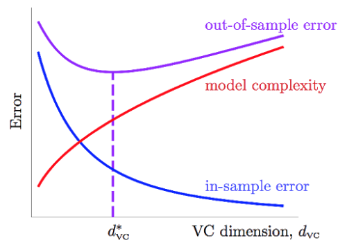
\[E_{\text{out}}(g) \le E_{\text{in}}(g) + \underbrace{\sqrt{\frac{8}{N} \ln{\left(\frac{4(2N)d_{VC}}{\delta}\right)}}}_{\Omega(N,\mathcal H,\delta)} \tag{2.9}\]$\Omega(N,\mathcal H,\delta)$ in formula above represents penalty for model complexity, and from which we can see powerful $h$ is not always good. Based on it, we have VC-curve as follows:

